
In a world of cutting-edge tech, Microsoft Excel has stood the test of time as an essential piece of business software. From basic business accounting to the simple presentation of customer data, nothing has yet come close to competing with Microsoft's humble –yet powerful – spreadsheet application.
However, with number-crunching duties often left to somebody else, thousands of business owners will be unaware of the functions that make Microsoft Excel such a useful tool.
To save startups the expense of hiring a part-time accountant, we've created a step-by-step guide on the functions that will be of most value to a small business owner. Packed with screenshots and videos, we hope it will give you the confidence to take on some of the icky financial stuff yourself, at least in the early days.
A word of warning: this is a long article. If there are some functions that you already know, you can skip to the ones you don't by clicking on the relevant links below:
Conditional formatting
Conditional formatting allows you to format cells so that they appear differently when a certain value is entered. For example, a cell could be formatted to change colour if a specific word or numerical figure is written inside the cell.
Conditional formatting is commonly used to display results in an understandable way. In a business context, it can help managers to assess performance quickly and easily.
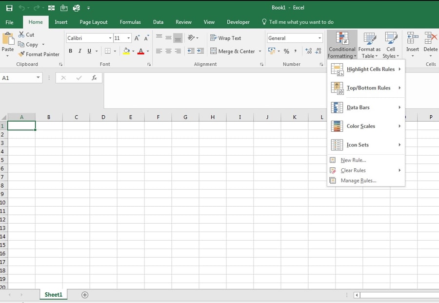
The conditional formatting section in Excel contains a number of options, as shown in the below screenshot.
Highlight cell rules
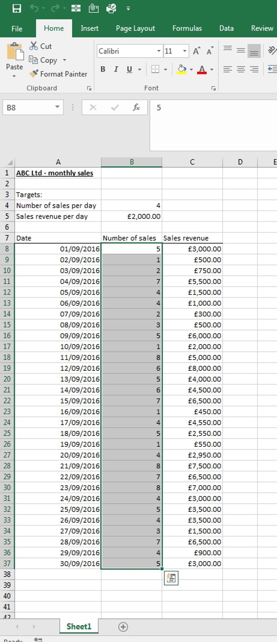
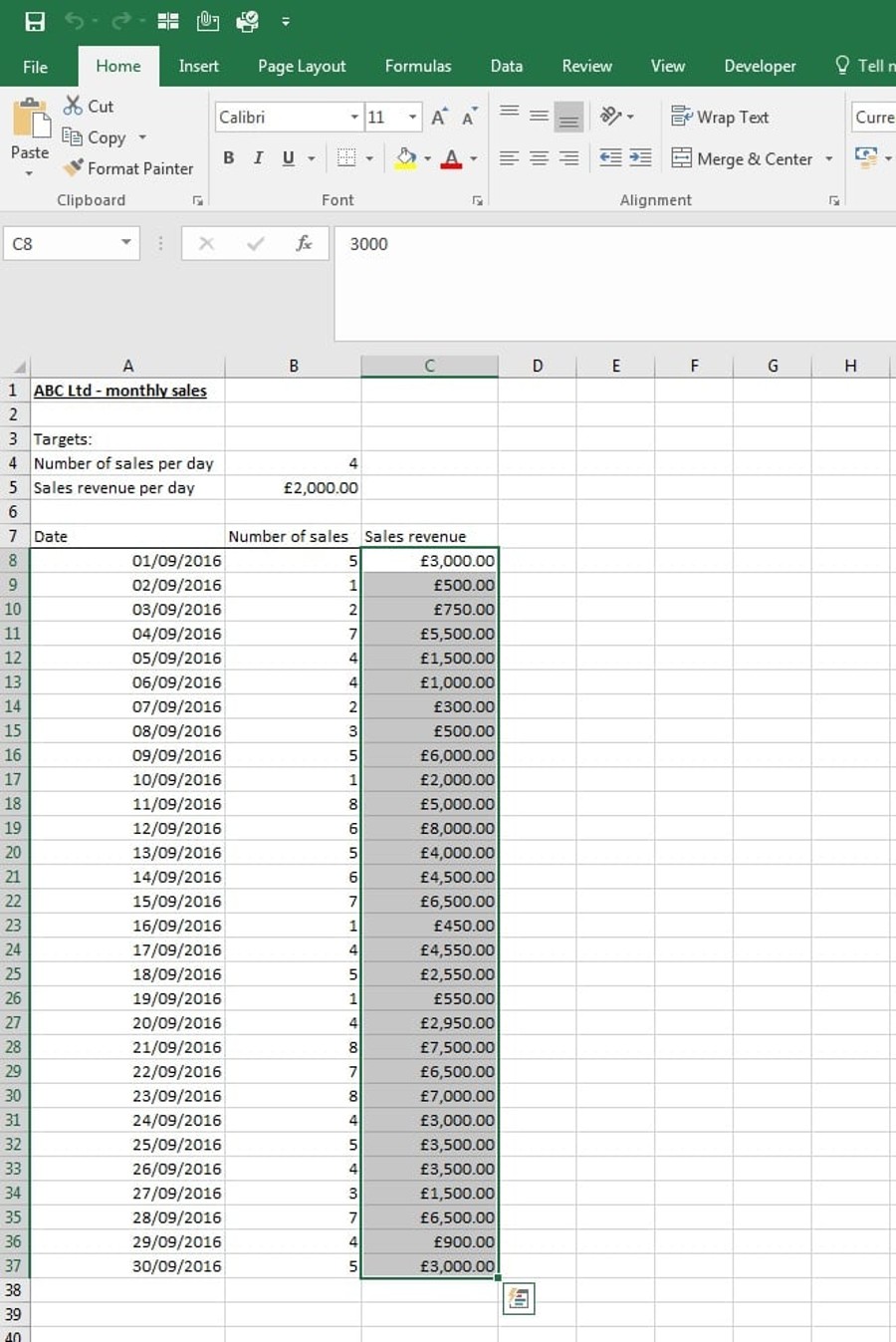
Using this function, you can set cells to be highlighted if they meet certain criteria. In this example, I want all of the cells where the target has been achieved to be highlighted in green.
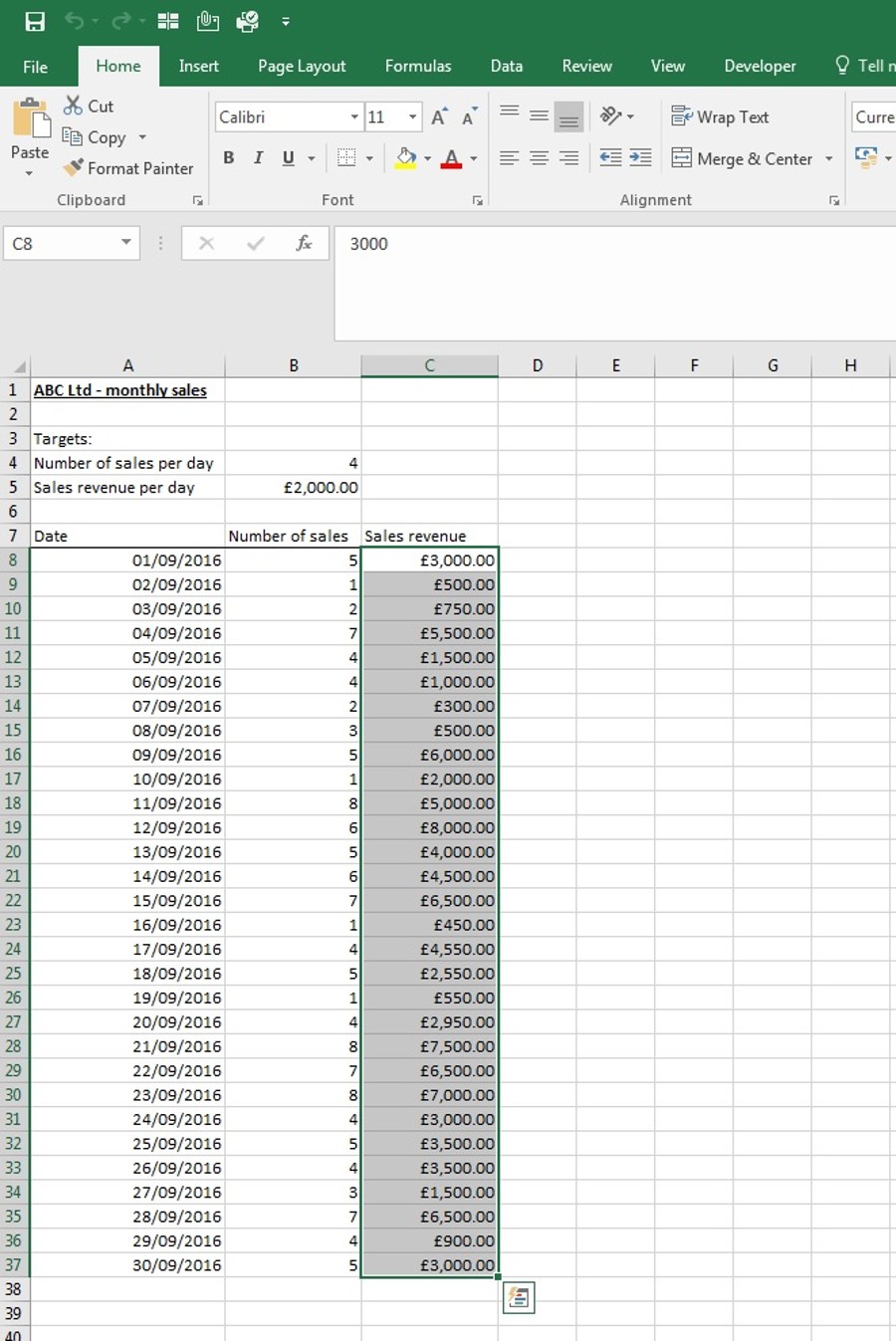
Step 1: Select the cells that you would like formatted.
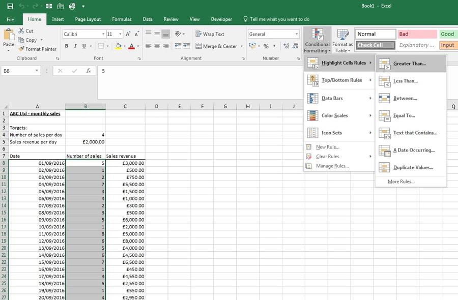
Step 2: Click on ‘Conditional Formatting’, ‘Highlight Cells Rules’, then ‘Greater Than’.
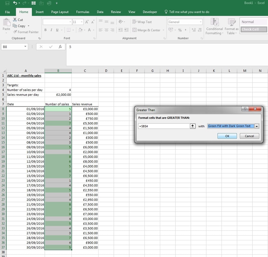
Step 3: Enter the rule in the pop-up box. In this example, we want the cells that are greater than the target to be highlighted. Select cell B4 (which contains the target) and choose the required formatting from the drop-down list.
We've also put together a video, so you can see this process from start to finish. This can be viewed below.
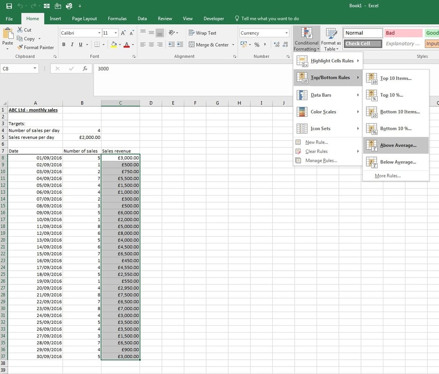
Top/bottom rules
Using this function, you can set cells to be highlighted when they meet a certain threshold.
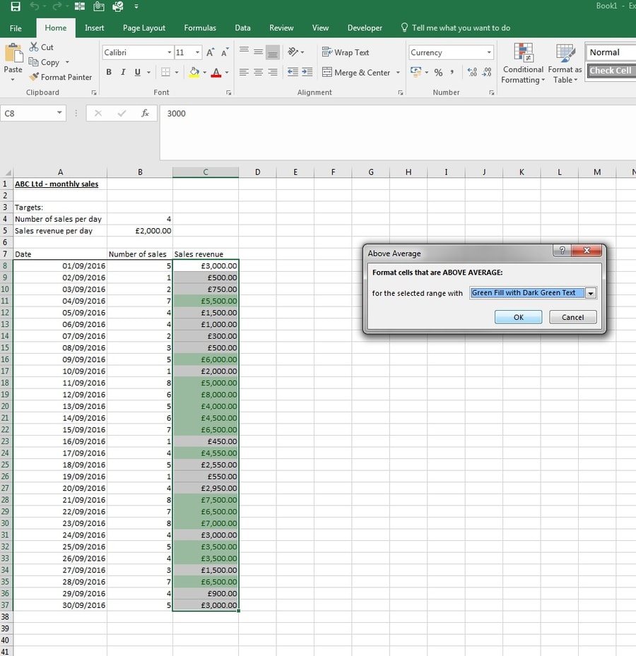
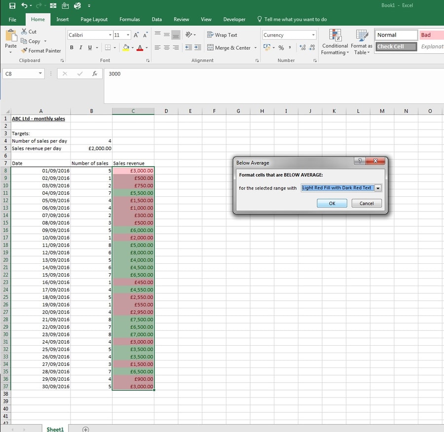
In this example, I want the cells where sales revenue is above average to be highlighted in green and the cells where sales revenue is below average to be highlighted in red.
Step 1: Select the cells that you would like formatted.
Step 3: Select the required formatting.
Step 4: Repeat the steps but instead use the ‘Below Average’ option.
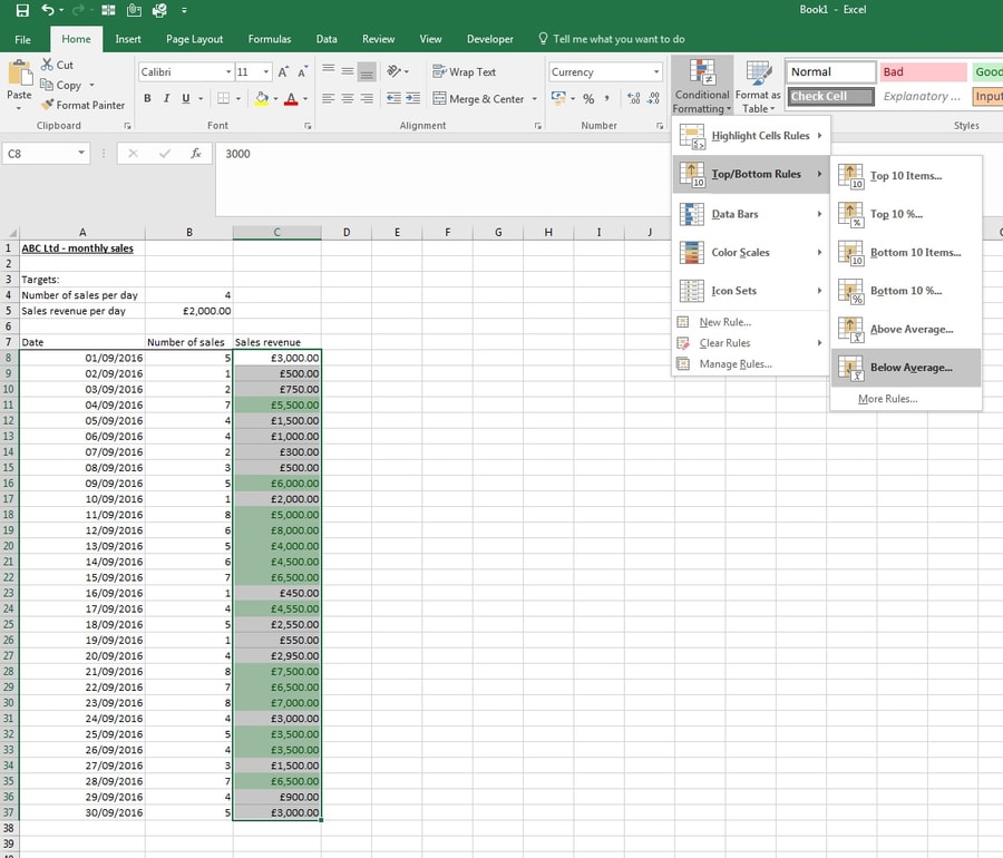
Watch the below video to see every step back-to-back.
Data bars/colour scales
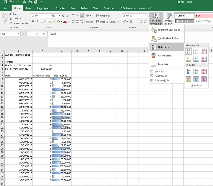
Data bars and colour scales allow your data to be displayed based on its values, and in a more visual way.
Data bars
Step 1: Select the cells that you would like formatted.

Step 2: Click on ‘Conditional Formatting’, then ‘Data Bars’.
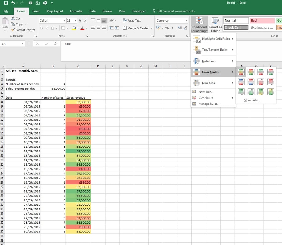
Colour scales:
Step 1: Select the cells that you would like formatted.
Step 2: Click on ‘Conditional Formatting’, then ‘Colour Scales’. Choose the required scale – here I have green-yellow-red where the highest figures are in green and the lowest in red.
And here's your video:
Pivot tables
A pivot table enables you to analyse large sets of data by displaying it in a clear and simple way.
A business owner, for example, might benefit from using a pivot table to present their sales figures. The table will allow the data to be subtotalled by date, product, sales division and so on.
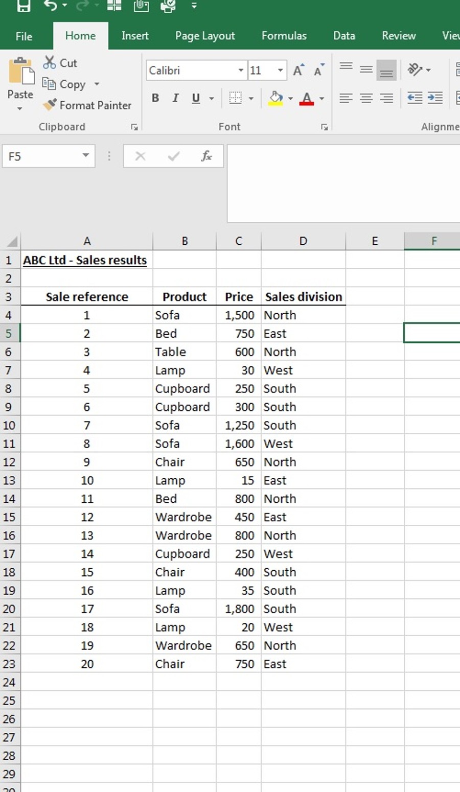
To illustrate how you can insert a pivot table into an Excel workbook, I am using the example company, ABC Ltd.
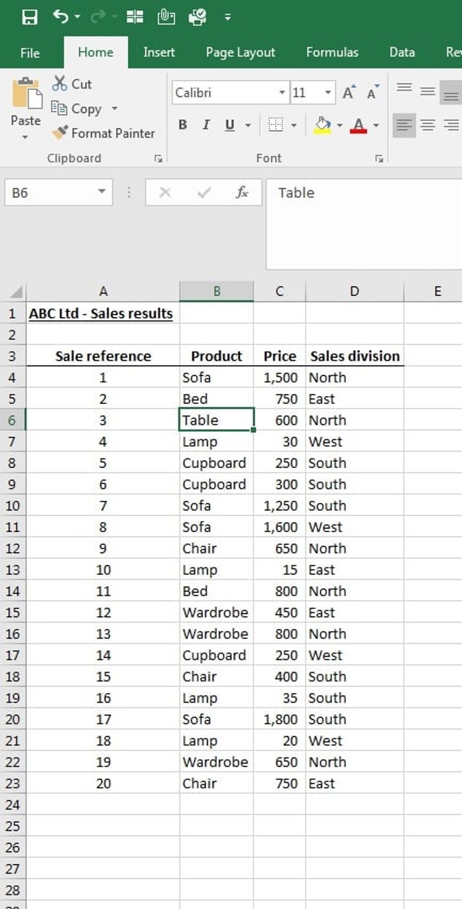
Step 1: Ensure that the data you are using is in columns with appropriate headings.
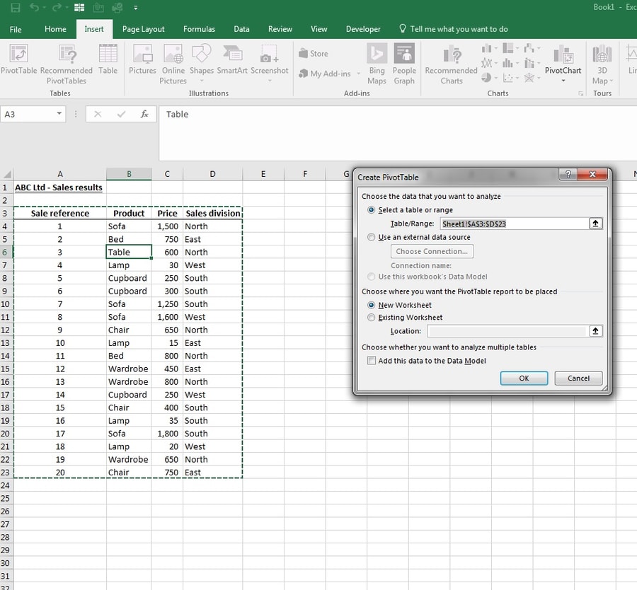
Step 2: Ensure that a cell within your data is selected, click on the ‘Insert’ tab, then ‘Pivot Table’.
Step 3: A ‘Create Pivot Table’ box will appear and your data should be highlighted by a dashed border. If you want the pivot table on a new worksheet within the same workbook then just click OK. If you would like it to be created in an existing worksheet, then select the option and the location, click where you would like the pivot table to be placed, and then click OK.
Step 4: The pivot table will appear, along with an options bar on the right-hand side of the workbook. The data columns are listed in the first box, with the four sections below letting you decide how your data will be displayed.
Filters: Drag a field to this section in order to filter all of the data in the table by a certain variable. For example, we could filter our pivot table by sales division.
Columns/Rows: Drag the fields to this section that you would like your data to be summarized by. For example, we could have rows by product type.
Values: Drag the fields to this section in order to total the values for each relevant row. For example, a sum of the prices that items were sold for. You can also summarize the values in ways other than SUM. Simply click the down arrow on the field that has been dragged into the ‘Values’ section in the right-hand bar, click on ‘value field settings’, then select how you would like the data to be summarized.
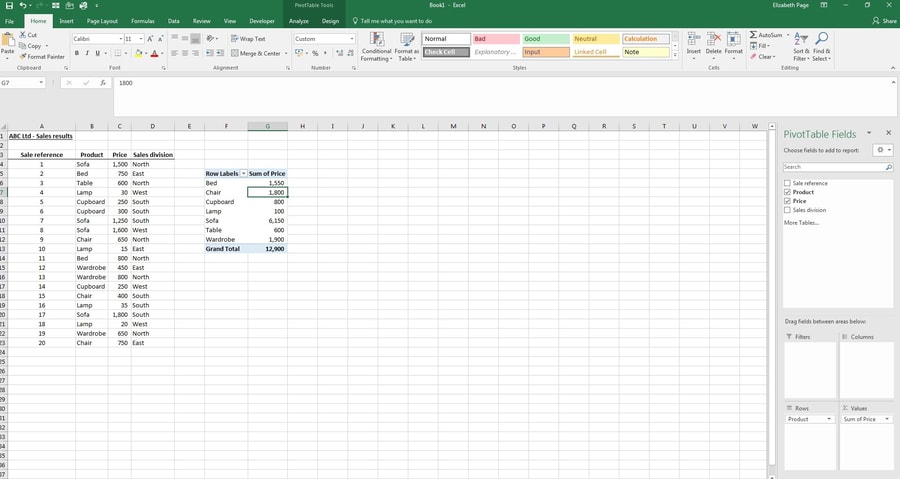
Step 5: Filter the pivot table as required to analyse the performance of each sales division.
SUM, IF, COUNT, SUMIF, COUNTIF
Excel has a range of functions that save you the trouble of reaching for a calculator. This section will run through each of them.
SUM
The SUM function totals the numbers in a range of cells. The easiest way to perform the SUM function is by using the ‘AutoSum’ button. Click into the cell where you would like the SUM to appear. Click on the AutoSum button in the home tab, select the required range of cells, then hit the enter or return key on your keyboard.

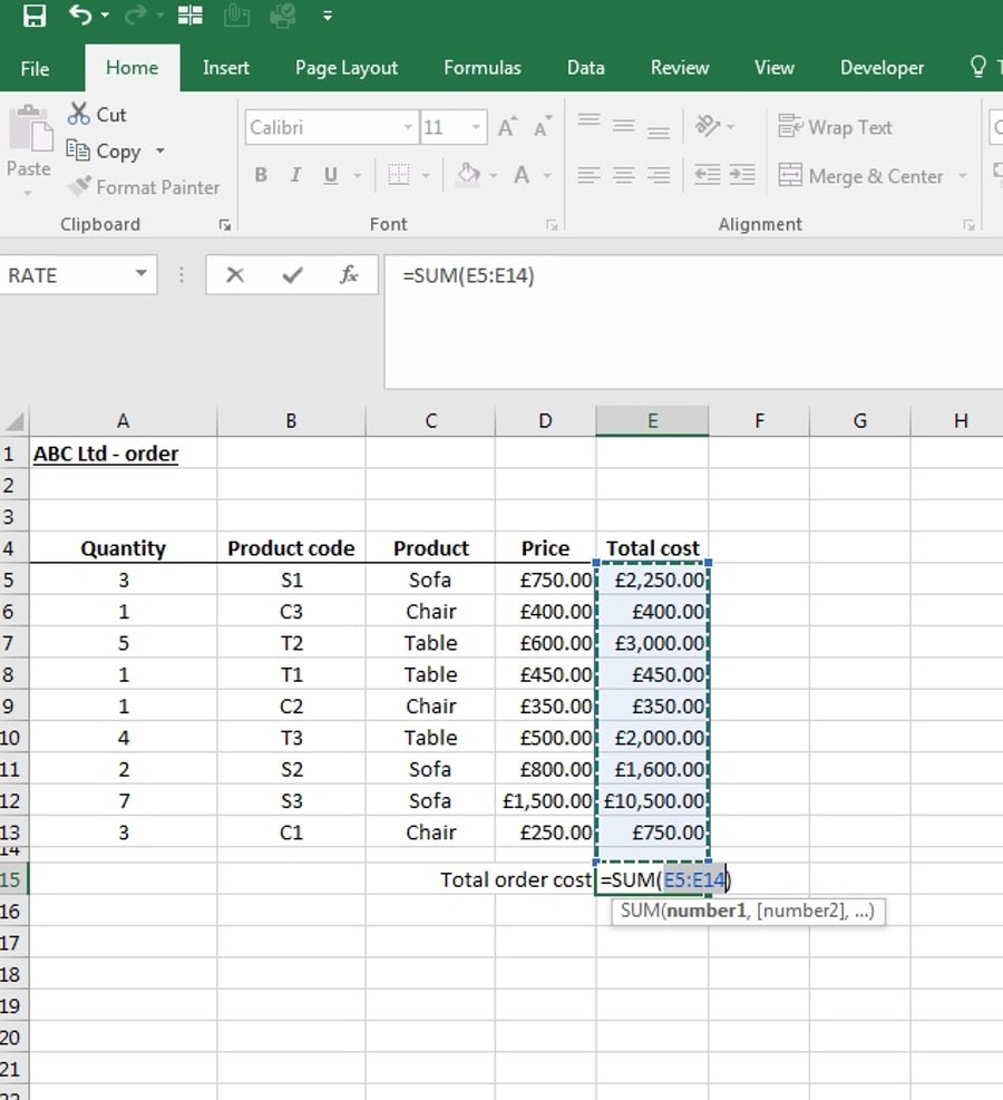
In addition to the two options above, you could also type =SUM( into the cell where you’d like the sum to appear, select the range of cells that you would like to total, then close the bracket.
COUNT
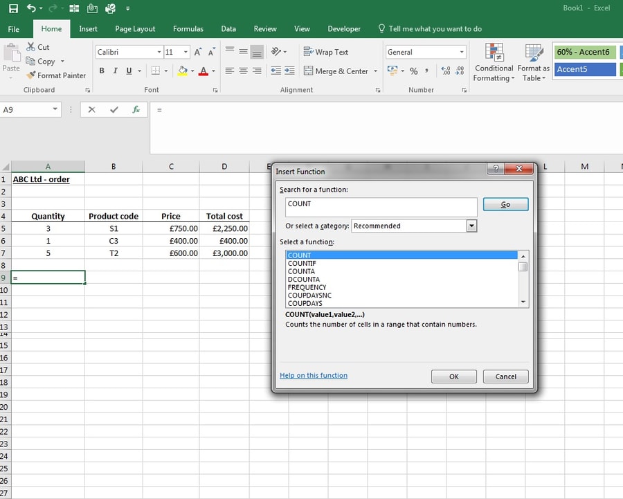
The COUNT function allows you to count the number of entries in a set of data.
In the following example, a COUNT function will be used to count the number of items in an order.
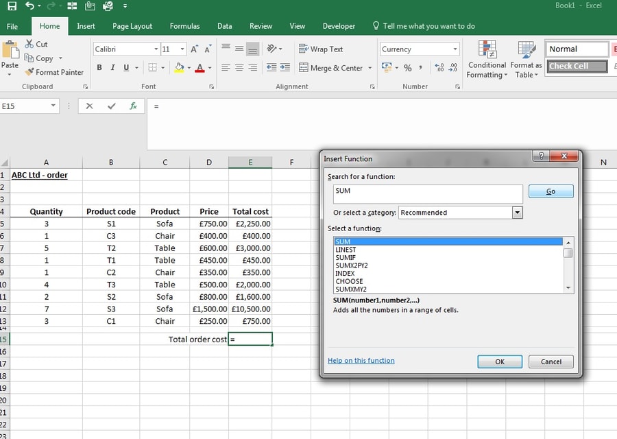
Step 1: Use the ‘insert function’ button and search for COUNT, then press OK.
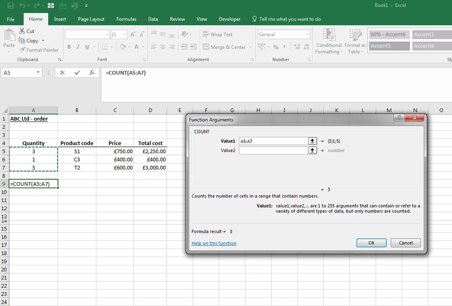
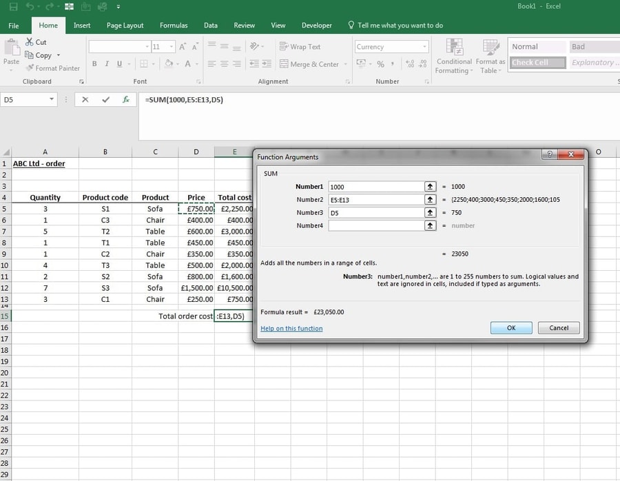
Step 3: If it is more than one column of data that you need counting, use the fields Value2, Value3 and so on.
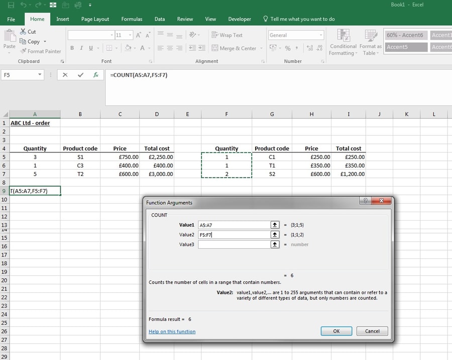
Step 4: Click OK, and your count should be displayed in the relevant cell.
IF
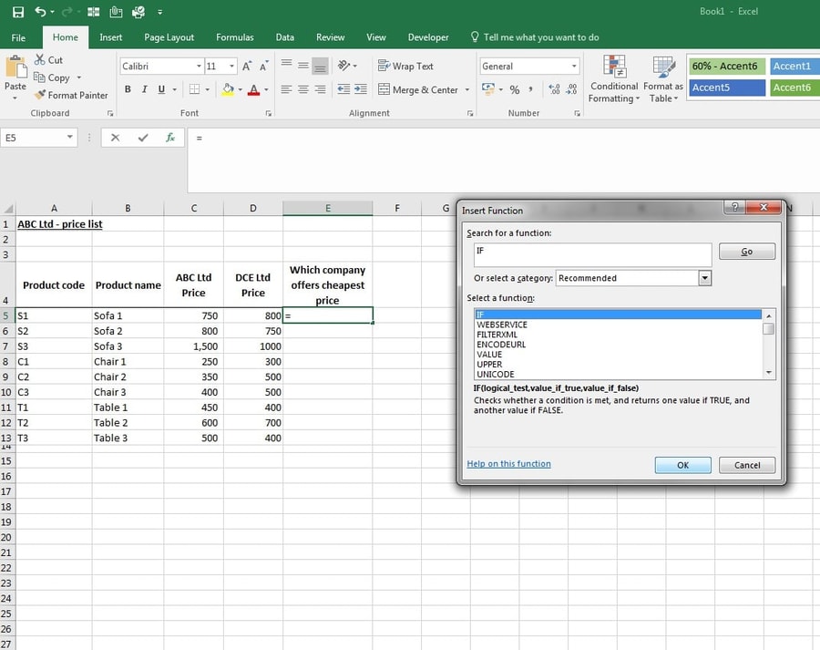
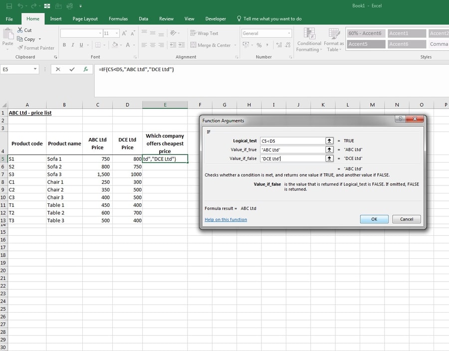
An IF function gives a result if a condition is true and another result if a condition is false. In this example, we will use the IF function to determine whether ABC Ltd or its competitor, DCE Ltd, is cheaper.
Step 1: Click the Insert Function button, search for ‘IF’, then click OK.
Step 2: You will see that there are three components to the formula.
The ‘Logical_test’ is the condition that can either be TRUE or FALSE. In this example, the condition is whether an ABC Ltd product is cheaper than the DCE Ltd product.
To set this as the condition, ‘C5<D5’ (the value of cell C5 is less than the value of cell D5) has been typed into the logical test box.
The ‘Value_if_true’ is the value you wish to be returned if the condition is true. In this case, if ABC Ltd is cheaper, we want ‘ABC Ltd’ to be returned.
The ‘Value_if_false’ is the value
you wish to be returned if the condition is false. In this case, if DCE Ltd is
cheaper, we want ‘DCE Ltd’ to be returned.
Step 3: Press OK, then drag the formula down to the end of the data list, so that it applies to all cells.
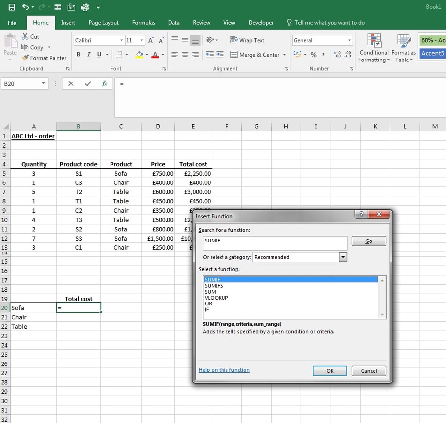
SUMIF
The SUMIF function totals the numbers in a range of cells if a condition is satisfied.
In the following example, a SUMIF function will be used to subtotal an order by product type.
Step 1: Use the ‘insert function’ button and search for SUMIF, then press OK.
Step 2: You will see that there are three components of this formula; the range, the criteria and the sum range.
The range is the group of cells that the criteria will be tested against. In this example, the range will be the range C5:C13, or products.
The criteria is the product type that you would like subtotalled. In this example, the criteria will be either Sofa, Chair or Table. Here you can either type in ‘Sofa’ or click on the cell A20, and so on.
The sum range is the group of cells that need to be subtotalled when the criteria is satisfied.
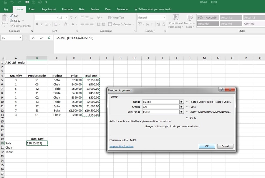
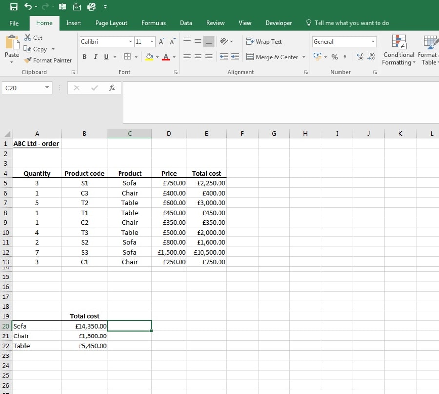
Step 3: Click OK, and repeat the process for the other product types. The subtotals should then be displayed in the relevant cells.
The video that walks you through all of the above is available to watch below:
COUNTIF
The COUNTIF function allows you to count the number of entries that satisfy a condition.
In the following example a COUNTIF function will be used to count the number of items in an order by item type.
Step 1: Use the ‘insert function’ button and search for COUNTIF, then press OK.
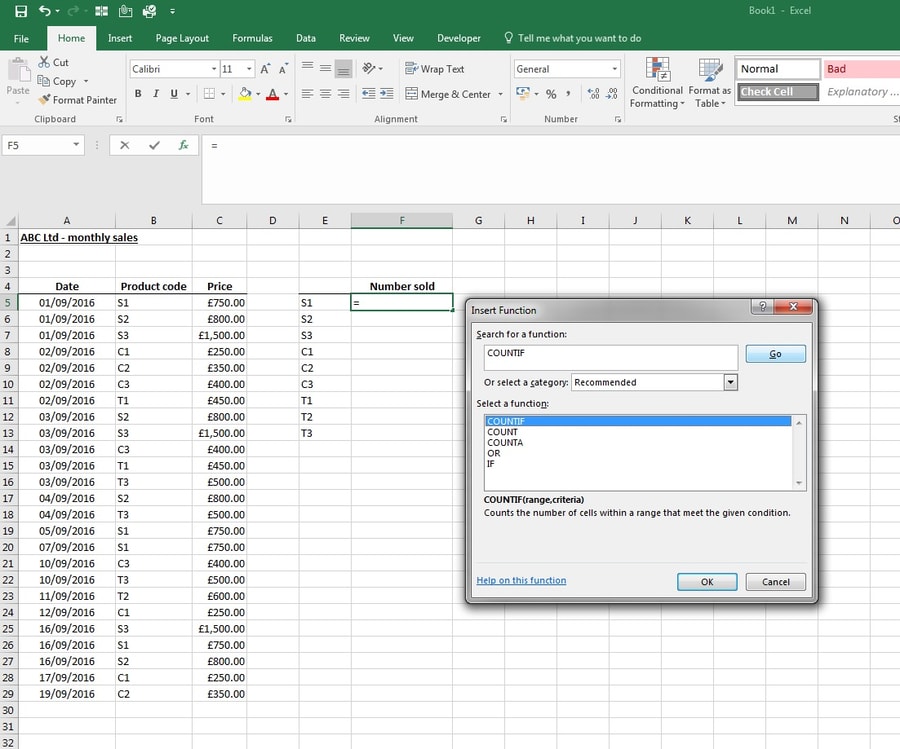
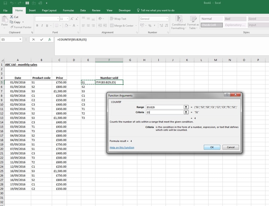
Step 2: There are two components to this function; the range and the criteria.
The range is the group of cells that the criteria will be tested against. In this example, the range will be the range B5:B29, or product code.
The criteria is what the range of cells (above) is evaluated against. In this example, the criteria will be the product code. Here you can either type in ‘S1’ or click on the cell E5.
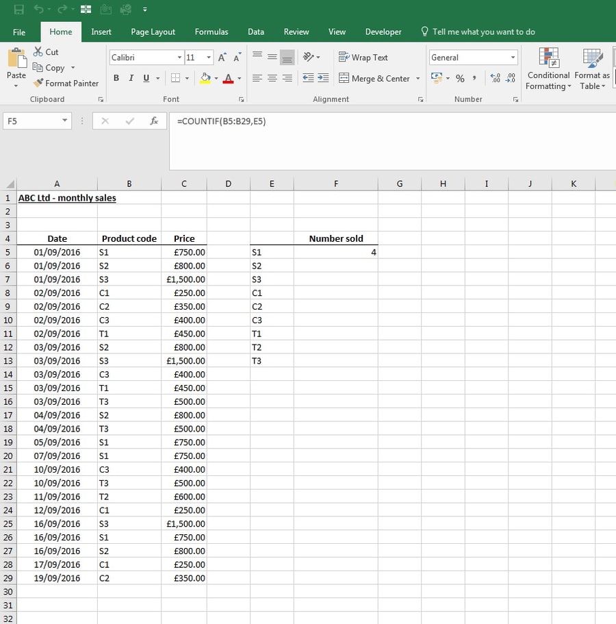
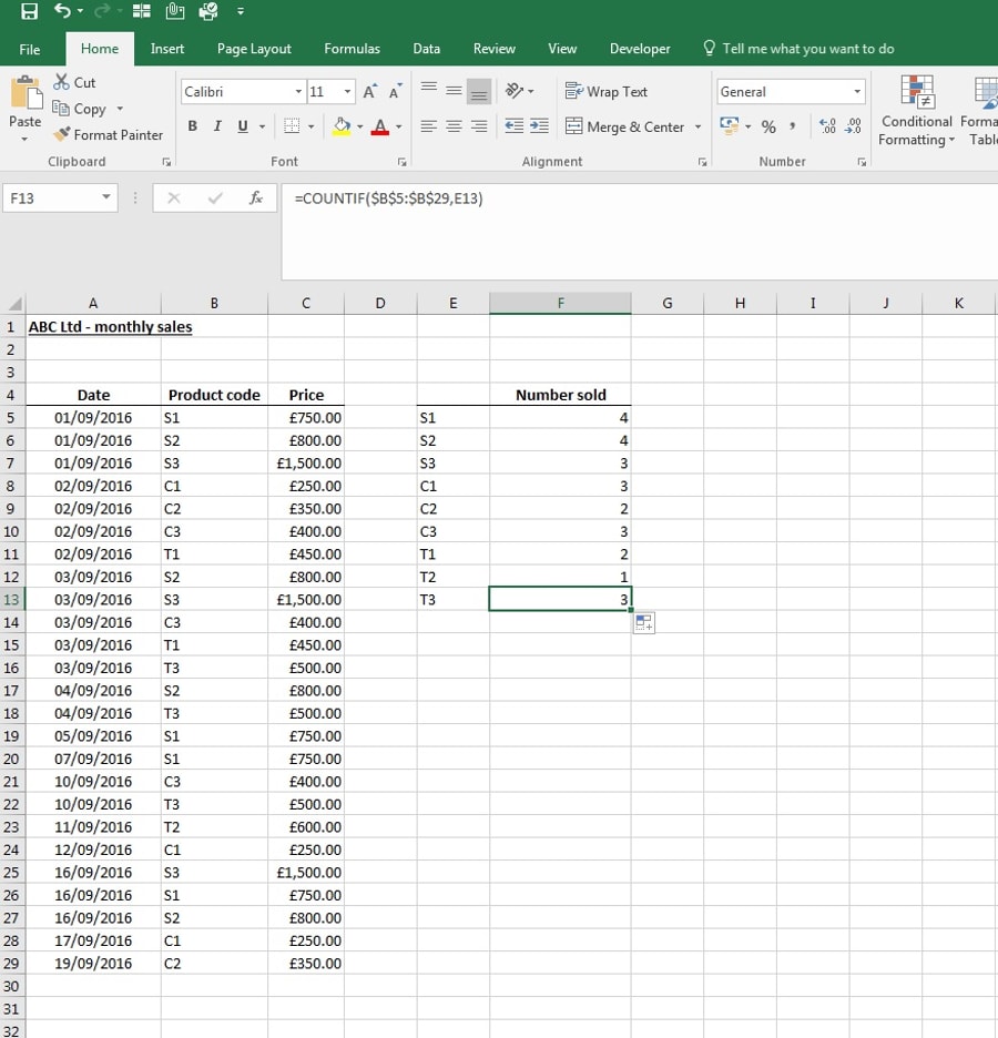
Step 3: Press OK, and your count should be displayed in the relevant cell.
Here's a step-by-step video tutorial for the COUNTIF function:
Vlookups
The Vlookup function is one of Excel’s most useful. When you have two sets of data and you need to pull information from one to another, a Vlookup is the ideal solution.
A Vlookup looks up a value in a vertical set of data and retrieves another item on the same row. For example, you may use a lookup to find a price of a product by using the product code.
Using company ABC Ltd, the below steps illustrate how to perform a Vlookup.
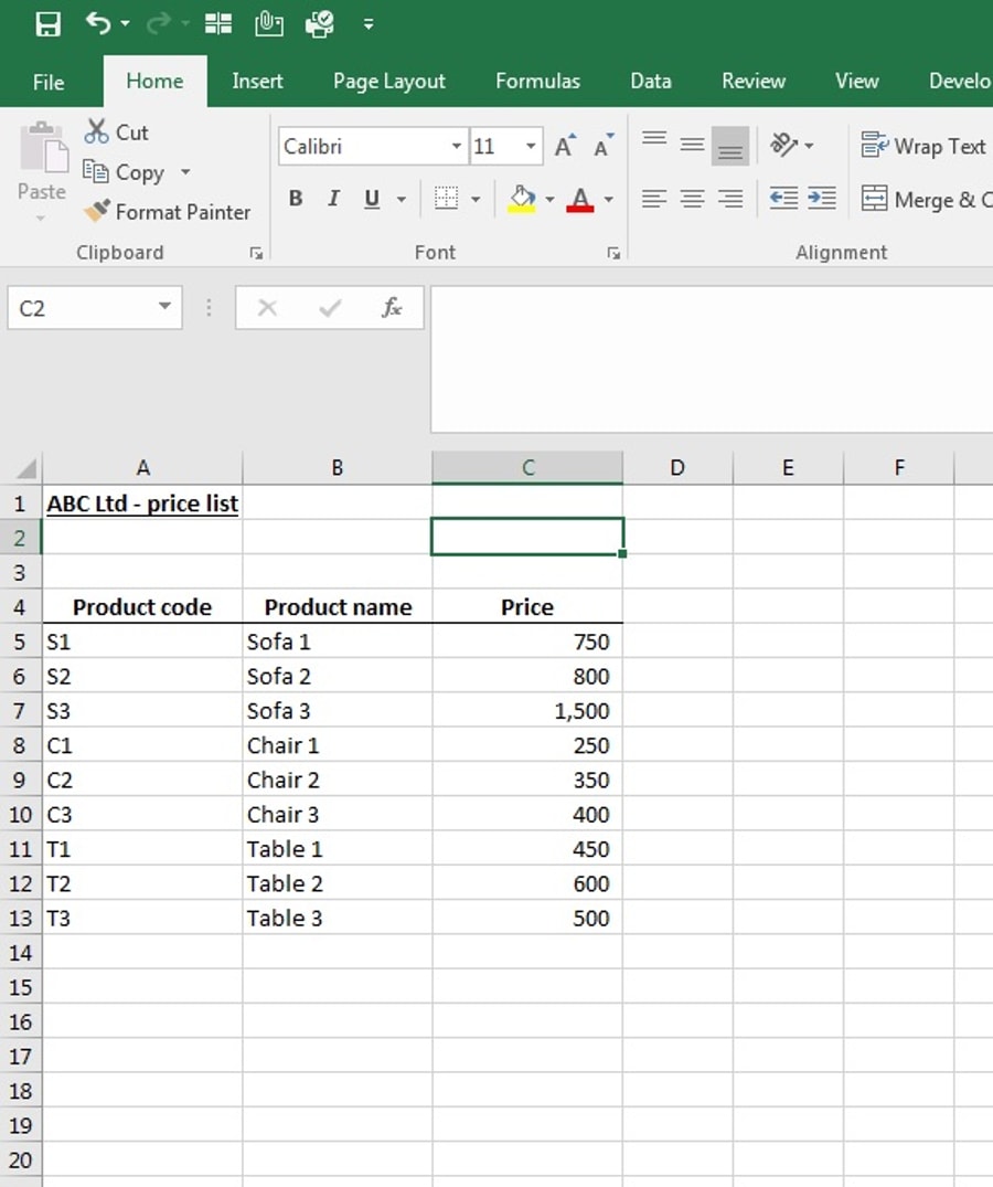
Step 1: You can use a Vlookup to look data up from sheets in the same workbook or separate workbooks. In this example, I will be using two sheets from the same workbook.
The first shows the price list for ABC Ltd. The second lists the items and quantities of a sales order.
Note: my example only uses a small amount of data. Vlookups become even more useful for large data sets.
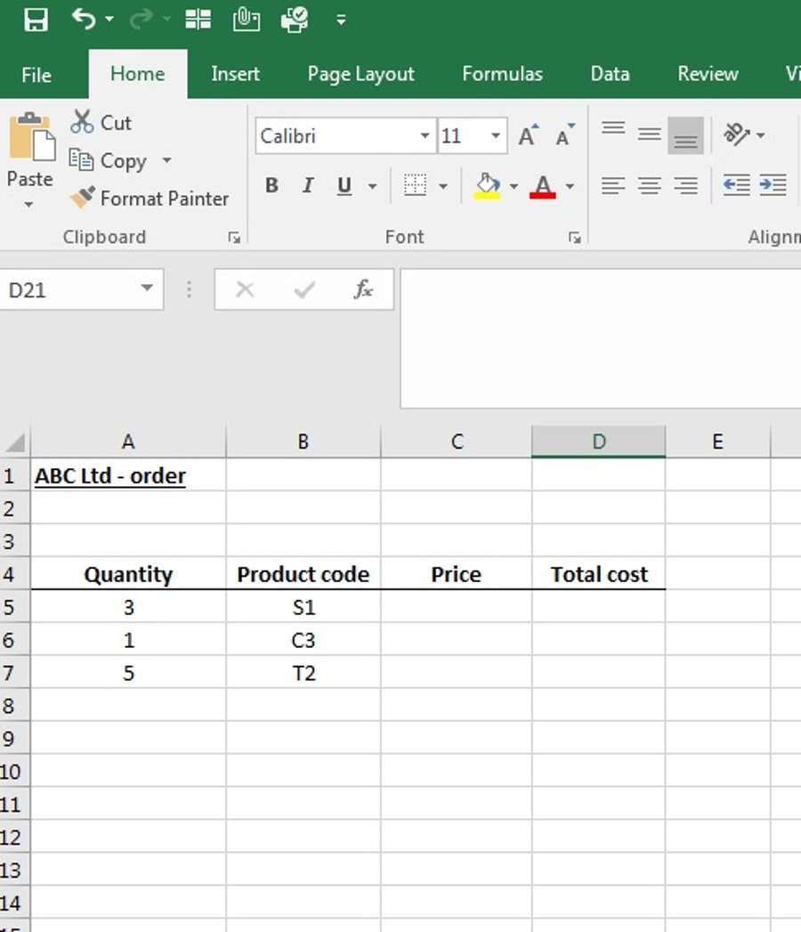
For this example, we want to look up the price for each product from the price list and add these to the order to calculate the total cost of the order.
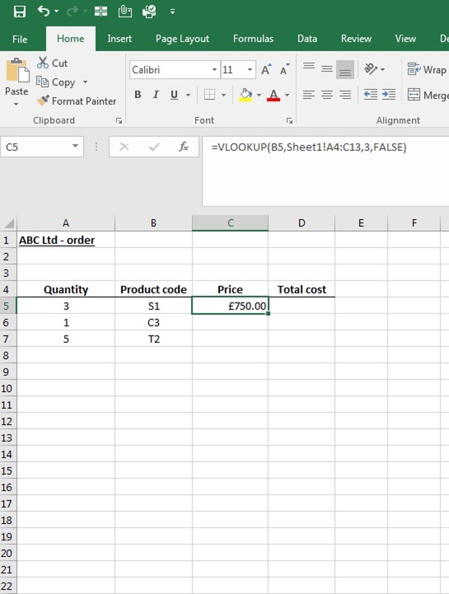
Step 2: Click on the cell where you require the data to be populated to – in this case, column C (price) on the order sheet.
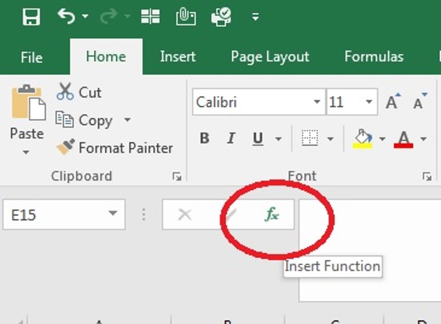
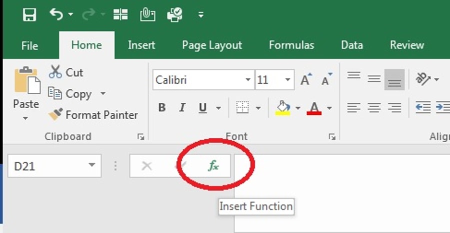
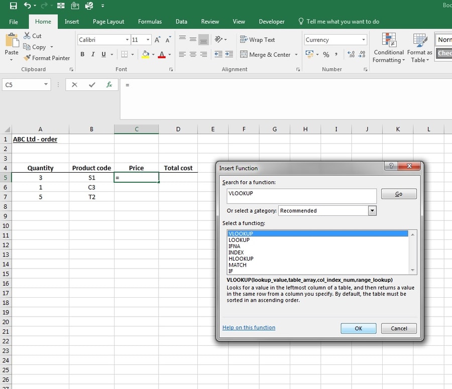
Click on the ‘insert function’ button, which is circled in red below, and search ‘vlookup’. Click on ‘vlookup’ and click OK.
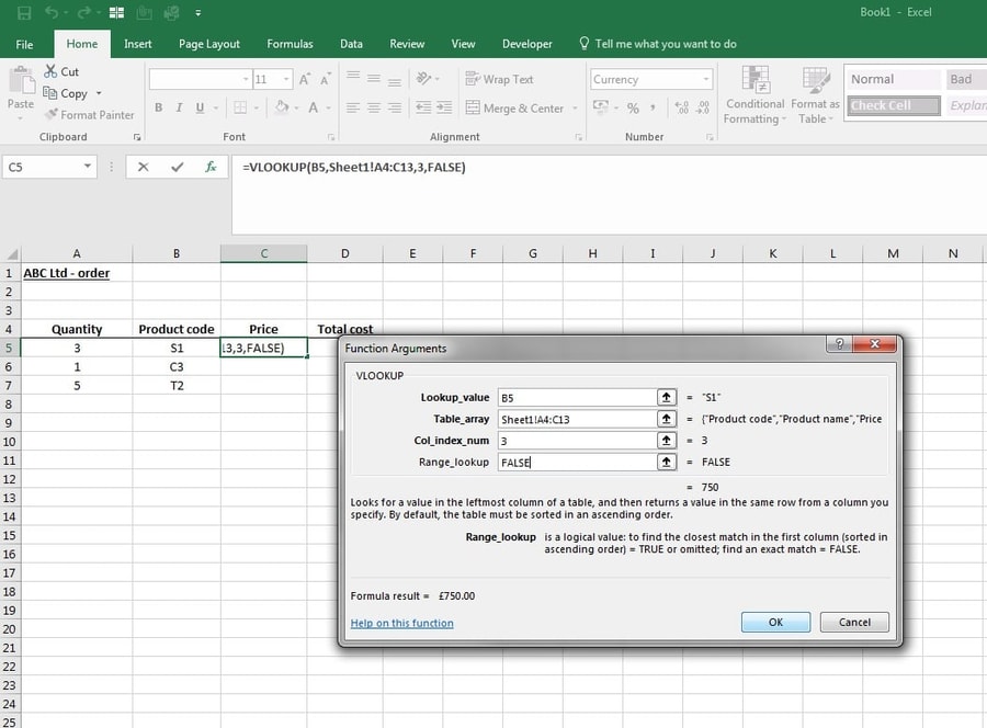
Step 3: The ‘function agreements’ box will appear.
The ‘lookup value’ is the value that you want to find in the other set of data. In this case, the product code.
The ‘table array’ is the table of data in which you are looking for the value. In this case, the price list.
The ‘column index number’ is the column number in the table that contains the data you are looking up.
The range lookup is either TRUE or FALSE, TRUE to find the closest match in a set of data or FALSE to find an exact match.
Complete the box as follows:
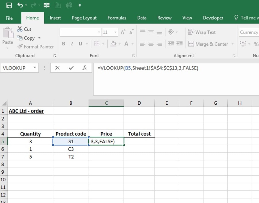
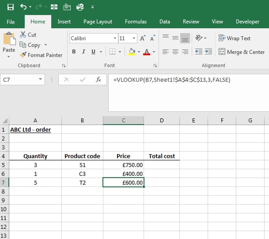
Rather than repeating this step for each product, you can simply copy the formula into the cells below.
Note: When copying the vlookup to the rows below, Excel automatically adjusts the formula to pick up the correct product code. E.g. when copying the formula into cell C6, the formula will adjust to look up the product in cell B6. However, it also adjusts the table array, which may cause an issue by missing data. In order to look up in the same table, you can enter $ around the cells which will prevent Excel from adjusting these cells. This is called an absolute reference.
Before copying the lookup formula to rows 6 and 7, change the formula to the following:
=VLOOKUP(Order!B5,'Price List'!$A$4:$C$13,3,FALSE)
And here it is: your last video.
Congratulations, you're now an Excel whizz. Feels pretty good, right? Although you might eventually need to hire an accountant, hopefully you can crunch those all-important numbers on your own for the time-being.
You may even want to share your spreadsheet skills with your friends and colleagues. We reckon they'll be well impressed. Alternatively, if you're too busy (or lazy), just point them to this article. It's entirely up to you.


These cookies are set by a range of social media services that we have added to the site to enable you to share our content with your friends and networks. They are capable of tracking your browser across other sites and building up a profile of your interests. This may impact the content and messages you see on other websites you visit.
If you do not allow these cookies you may not be able to use or see these sharing tools.